Multiple Regression and Logistic Regression in R
Bhanji - Statistical Methods
2024-02-21
Goals for today
Learn how to use linear regression with one continuous outcome and one or more predictors
use scatterplots to check for non-linear associations
understand model R2, F-statistic, beta coefficients (standardized, unstandardized)
check model residuals for potential sources of bias
- linearity, homoscedasticity, independence, normality and extreme cases
F-statistic for model comparisons
Examine curvilinear/quadratic associations (this wasn’t in the SPSS activity)
- understand multi-collinearity and indicators (tolerance, VIF)
Dichotomous outcome: logistic regression
- why not use regular linear regression?
- sigmoid link function (logit)
- interpret coefficients as log-odds
- why not use regular linear regression?
Starting off notes
Step 1 - Get organized
- Now open RStudio and start a new project, select “Existing
Directory” and select the folder you created for this activity
- Earlier you downloaded lumos_subset1000plusimaginary.csv
- In RStudio, start a new R markdown and do your work in there, save
the file in a subfolder called r_docs
put these lines in your “setup” code chunk:
knitr::opts_chunk$set(echo = TRUE)
knitr::opts_knit$set(root.dir = rprojroot::find_rstudio_root_file())
library(tidyverse)run the setup code chunk (the necessary
library()statements are in there)
- In the RStudio console, install the packages you’ll need today with
the install.packages() command:
install.packages("GGally")
install.packages("parameters")
Step 2 - Import data and check it out
data description: lumos_subset1000plusimaginary.csv is the same file we worked with last week. This is subset of a public dataset of lumosity (a cognitive training website) user performance data. You can find the publication associated with the full dataset here:
Guerra-Carrillo, B., Katovich, K., & Bunge, S. A. (2017). Does higher education hone cognitive functioning and learning efficacy? Findings from a large and diverse sample. PloS one, 12(8), e0182276. https://doi.org/10.1371/journal.pone.0182276- this data subset includes only the arithmetic reasoning test (AR)
score from a post-test at the end of a 100 day training program
(
raw_score)
pretest_score(test at start of the training program) has been transformed to have a mean of 100 and standard deviation of 15 (this is a typical transformation for IQ scores)
- this data subset includes only the arithmetic reasoning test (AR)
score from a post-test at the end of a 100 day training program
(
What to do first: Make a new code chunk and use readr::read_csv() to read in the data. Make sure that NA values are handled the way you want (click on the tibble in the Environment window pane to take a quick look).
What to do next: make sure the columns that contain nominal vals are treated as nominal, using forcats::as_factor() you can copy your code chunk from last week, or just look at the solution below
#first import the data
lumos_tib <- readr::read_csv("data/lumos_subset1000plusimaginary.csv", na = "NA")
# now make sure the columns we want as factors are treated that way, using forcats::as_factor()
lumos_tib <- lumos_tib %>% dplyr::mutate(
  test_type = forcats::as_factor(test_type),
  assessment = forcats::as_factor(assessment),
  gender = forcats::as_factor(gender),
  edu_cat = forcats::as_factor(edu_cat),
  english_nativelang = forcats::as_factor(english_nativelang),
  ethnicity = forcats::as_factor(ethnicity)
)
Step 3 - The General Linear Model (GLM) with one predictor
A note about terminology: (same as the note in the SPSS activity) In this lab activity we will use the terms “predictor”, “independent variable (IV)”, and “explanatory variable” interchangeably to refer to variables that are entered as explanatory terms in the model. We will use the terms “dependent variable” and “outcome variable” interchangeably to refer to the variable that is being explained. You should be mindful of the implications of these words (e.g., about causality, which cannot be inferred simply by assigning one variable as a predictor and another as an outcome) but we won’t focus on language in this lab. Instead, you should get used to the different terminology that is used.

Above is the decision process chart from the book.
- It says we should start by using scatter plots to check for non-linear associations and unusual cases.
- Last week we looked at scatter plots of pretest_score, raw_score,
and age. The linearity assumption was reasonable and there were no
concerning outliers, but let’s use a shortcut to recreate those scatter
plots all at once. Use the function
GGally::ggscatmat()like in the code below.
p1 <- lumos_tib %>%
  GGally::ggscatmat(columns = c("age","pretest_score","raw_score"))
## Registered S3 method overwritten by 'GGally':
## method from
## +.gg ggplot2p1
- Notice that the age variable is not normally
distributed, but normality of the variables, especially with a large
data set is not a concern. The scatters show that a linear relation
between variables is a reasonable assumption
- So let’s dive straight in and use linear regression with
age as an explanatory variable for
raw_score
- We will use the lm() function, piping in the data and
specifying age as a predictor for raw_score
with the argument formula = raw_score ~ age (an intercept
term is automatically included). Save the model in a variable called
score_lm
- use summary(score_lm) to show the model summary
score_lm <- lumos_tib %>% drop_na(age,raw_score) %>%
  lm(formula = raw_score ~ age)
summary(score_lm)
##
## Call:
## lm(formula = raw_score ~ age, data = .)
##
## Residuals:
## Min 1Q Median 3Q Max
## -16.8899 -3.4962 -0.0183 3.1838 21.1927
##
## Coefficients:
## Estimate Std. Error t value Pr(>|t|)
## (Intercept) 17.83974 0.58027 30.74 < 2e-16 ***
## age -0.04130 0.01282 -3.22 0.00132 **
## ---
## Signif. codes: 0 '***' 0.001 '**' 0.01 '*' 0.05 '.' 0.1 ' ' 1
##
## Residual standard error: 5.003 on 998 degrees of freedom
## Multiple R-squared: 0.01028, Adjusted R-squared: 0.009291
## F-statistic: 10.37 on 1 and 998 DF, p-value: 0.001323Looking at the model summary:
- The Multiple R-squared value tells us that
ageexplains about 1.03% of the variance inraw_score(not much by most standards).
- The F-statistic is the ratio of variance explained by the model to
the error within the model (use
anova(score_lm)to view Mean Sum of Squares for the model and residuals), and the p-value tells you the probability of an F-statistic at least that large under the null hypothesis. - The (unstandardized) beta coefficient (“Estimate” column, “age” row)
tells you that a change of one unit in the predictor (age) predicts a
change of -.04 units in the outcome (raw_score). In other words, the
model predicts that two people one year apart in age will be .04 units
apart in their performance score (the older person having the lower
predicted score).
- you can get standardized coefficients by using the command
parameters::model_parameters(score_lm, standardize="refit")(this function also gives you confidence intervals for parameters)- the standardized coefficient forageindicates that a change of +1 standard deviation in age predicts a change of -.10 standard deviations inraw_scoreit is the same as if we first standardized (z-scored) each variable and then ran the regression model.
- The Intercept (“Estimate” column, “(Intercept)” row) tells us that
if all predictors were at their zero level (i.e., at age zero) the model
predicts a score of 17.84. It doesn’t make a lot of sense to talk about
a score for someone age zero, but this is how linear models work. If you
wanted an interpretable intercept you could re-scale
ageso that the zero value was meaningful (e.g., re-center to mean=0, then the intercept would correspond to the predicted score for someone with the mean age)
- The “Std. Error” column gives the standard error of each estimate
(intercept and age coefficient) – for a visual explanation of standard
error of regression coefficients, see the Andy Field video on the topic (same
as the one in the syllabus).
- The “t value” column gives the t-stat for each estimate
(estimate/std err) and the “Pr(>|t|)” column gives the probability of
observing a t-stat that far from zero under the null hypothesis.
- notice that the p-value for
age(under “Pr(>|t|)”) is the same as the overall p-value - this is because age is the only predictor in the model - notice that the t-stat and p-value for
ageare the same as the t-stat and p-value the we got last week for the correlation betweenageandraw_score- this is because the correlation is also a test of a linear relation (andageis the only predictor)
Step 4 - The General Linear Model (GLM) with multiple predictors
Now let’s add pretest_score to our model, so that we are
predicting raw_score as a function of age and
pretest_score. See if you can write the code yourself (copy
and edit the code from the previous step) before looking at the solution
below. Store the model in a variable named
score_2pred_lm.
score_2pred_lm <- lumos_tib %>% drop_na(age,raw_score,pretest_score) %>%
  lm(formula = raw_score ~ age + pretest_score)
summary(score_2pred_lm)
##
## Call:
## lm(formula = raw_score ~ age + pretest_score, data = .)
##
## Residuals:
## Min 1Q Median 3Q Max
## -11.7387 -2.0523 0.0005 2.1198 9.3891
##
## Coefficients:
## Estimate Std. Error t value Pr(>|t|)
## (Intercept) -11.904994 0.846546 -14.063 <2e-16 ***
## age -0.005794 0.008131 -0.713 0.476
## pretest_score 0.274721 0.007052 38.956 <2e-16 ***
## ---
## Signif. codes: 0 '***' 0.001 '**' 0.01 '*' 0.05 '.' 0.1 ' ' 1
##
## Residual standard error: 3.152 on 997 degrees of freedom
## Multiple R-squared: 0.6076, Adjusted R-squared: 0.6068
## F-statistic: 771.9 on 2 and 997 DF, p-value: < 2.2e-16
Now, answer the following questions for yourself based on the model summary
- What does the “Multiple R-squared” tell you for this model? That is,
what percent of the variance in
raw_scoreis explained by the model? - What does the overall F-statistic and p-value tell you?
- What does the beta coefficient for
pretest_scoretell you?
- What does it mean that the t-statistic for the
agevariable is not significant in this model? How does it compare to the partial correlation test that we ran last week with the same variables?
Step 5 - Model diagnostics: Examine model residuals for potential sources of bias
- Aside from the model summary information, when you fit a linear
regression model, the
lm()function produces a predicted outcome value for every set of predictor variables (e.g., if one participant has an age of 15 and a pretest_score of 99.3 then the predicted outcome value will be 17.84 + (-.006*15) + (.275*99.3), based on the model we just estimated.
- The model residuals are the difference between each
predicted score and the actual outcome value (
raw_score), thus there are as many model residual values as there are cases. We’ll look at these residuals in this step
Now, look back at the decision process chart. It says we should look at “zpred vs zresid” to check for linearity, heteroscedasticity, and independence, then look at a histogram of residuals to check for normality.
Fortunately, there is one easy function that will show everything we
need: plot(modelname) - Use
plot(score_2pred_lm) to show the diagnostic plots for the 2
predictor model from the last step.
plot(score_2pred_lm)


Here is a brief description of each plot
- “Residuals vs. Fitted” - this is the unstandardized version of “zpred vs zresid” and is just as useful for checking linearity, heteroscedasticity, and independence. We are basically checking to make sure there are no clear patterns in the residuals.
- Here are some examples of patterns you might see in residuals that indicate sources of bias (from Prof Andy Field’s discovr tutorial section 08 - note that the non-linear example is also an example of non-independence, because the residuals are related to the fitted values.)
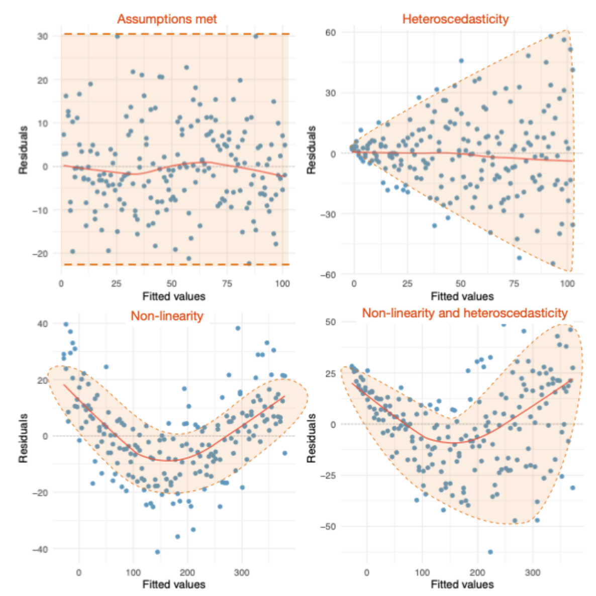
- “Normal Q-Q” - this is a Q-Q plot of the residuals, and helps us
check for non-normally distributed residuals. We expect points to fall
close to the dotted line if the residuals are normal (they do
here).
- “Scale-Location” - similar to the first plot, but the y-axis is the
square root of the absolute value of residuals. Use this for checking
linearity, heteroscedasticity, and independence along with the first
plot - they contain the similar information but some heteroscedastic
patterns may be more apparent in one plot or the other. See BoostedML
for more examples of heteroscedasticity.
- “Residuals vs Leverage” - Points with high leverage are cases that are potentially influential because of their extreme values. Here, we are checking (1) that the spread of residuals does not change across leverage values (approximately horizontal solid red line indicates no heteroscedasticity concern), and (2) that there are no points with very high influence (points outside the dotted red line, which is not visible in this case because there are no high leverage points), which would violate linearity. We saw an example of high leverage last week in Anscome’s Quartet Plot 4.
Step 6 - Compare Models
We can compare two models (w/ the same outcome data) by computing an
F-statistic based on the ratio of error (RSS=residual sum of squares) of
one model to the other (for example, a full model with all predictors
compared to less full model with a subset of predictors). If one model
is better at explaining the outcome than the other, than the RSS of the
worse model will be greater than the RSS of the better model, and the
F-statistic quantifies that for us (and gives a p-value under the null
hypothesis). You can also rephrase this F-statistic as a ratio based on
R2 for each model (see Chapter 9 of the Field Textbook,
equation 9.18)
- Let’s compare the last model (age and
pretest_score) to the first model (age only)
of raw_score. Because we are comparing the residual
variance between models, we can use the anova() function in
R. The arguments we pass are the names of the two models (put the fuller
model second). Try it now.
anova(score_lm, score_2pred_lm)## Analysis of Variance Table
##
## Model 1: raw_score ~ age
## Model 2: raw_score ~ age + pretest_score
## Res.Df RSS Df Sum of Sq F Pr(>F)
## 1 998 24978.7
## 2 997 9903.8 1 15075 1517.6 < 2.2e-16 ***
## ---
## Signif. codes: 0 '***' 0.001 '**' 0.01 '*' 0.05 '.' 0.1 ' ' 1
- The p-value tells us that the F-stat is unlikely under the null
hypothesis (that the models are equivalent). In other words, the
difference in variance explained by
age+pretest_scorevsagealone is unlikely if the models equally explain variance inraw_score(so the fuller model is better.
- When you report a model comparison this way you report the
F-statistic as well as the change in R-squared (R2 of better
model minus R2 of the worse model). But one important issue
is that adding more predictors will always increase R2.
- For this reason you may also report other indicators of model fit
that account for the number of predictors, such as AIC and BIC (see
Chapter 9 of the Field Textbook).
- You can view the AIC (Akaike Information Criterion) and BIC
(Bayesian Information Criterion) for each model by using
broom::glance(modelname)in R - lower AIC and BIC values indicate better model fit.
Step 7 - Quadratic/curvilinear associations
When we looked just at age and raw_score,
we saw a small association such that older participants scored lower.
But is it possible that the association is really inverted U-shaped such
that older is better at young ages, but worse at old ages? We can
examine this possibility by including a quadratic (age2) term
in the model. It’s as simple as centering the age variable (by
subtracting the mean) and squaring it, then including that term in the
model. It’s always best to include lower order terms when you add higher
order terms, so our new formula will be
raw_score ~ age_ctr + age_squared (first we have to compute
age_ctr and age_squared). Try it now: first
compute age_ctr and age_squared, then estimate
the model with the new formula (store the model in a variable named
score_agesq_lm).
lumos_tib <- lumos_tib %>%
  mutate(
    age_ctr = age-mean(age),
    age_squared = age_ctr^2
  )
score_agesq_lm <- lumos_tib %>%  lm(formula = raw_score ~ age_ctr + age_squared)
summary(score_agesq_lm)
##
## Call:
## lm(formula = raw_score ~ age_ctr + age_squared, data = .)
##
## Residuals:
## Min 1Q Median 3Q Max
## -16.5455 -3.4196 -0.0787 3.2473 21.3652
##
## Coefficients:
## Estimate Std. Error t value Pr(>|t|)
## (Intercept) 16.448005 0.243438 67.566 < 2e-16 ***
## age_ctr -0.059527 0.015266 -3.899 0.000103 ***
## age_squared -0.002668 0.001218 -2.191 0.028659 *
## ---
## Signif. codes: 0 '***' 0.001 '**' 0.01 '*' 0.05 '.' 0.1 ' ' 1
##
## Residual standard error: 4.993 on 997 degrees of freedom
## Multiple R-squared: 0.01503, Adjusted R-squared: 0.01305
## F-statistic: 7.605 on 2 and 997 DF, p-value: 0.0005273
Examine the model summary:
- Notice that there are coefficient estimates for
age_ctr, andage_squared.
- The “Multiple R-squared” is .015 - we can compare that to the model
that had age only (R-squared was .010), so the quadratic term increases
the variance explained just a little bit. The p-value for
age_squaredtells us that it is unlikely (p=.029) to find a t-stat this large under the null hypothesis (that the age_squared association is zero).
- You can go through the rest of the summary like before, but now let’s spare a moment to think about multi-collinearity.
Multi-collinearity (textbook Chapter 9, section 9.9.3)
- when predictors in the model are highly correlated with each other,
we have multi-collinearity and the estimates of coefficients
for correlated terms are unstable (large std err and highly variable
across samples)
- an easy way to check for multi-collinearity is by computing the
VIF (variance inflation factor) for each predictor. It measures
the shared variance between one predictor and the others. The reciprocal
of VIF is called tolerance. A general rule of thumb is that you
should worry if you have VIF > 5 for any predictor in the
model.
- check the VIF for each predictor now, by running
car::vif(score_agesq_lm)– looks okay, right? But what if we hadn’t centered the age variable before squaring it?
Step 8 - Dichotomous outcome: logistic regression
Logistic regression is used when the outcome variable has just two
possible values (e.g., true/false, on/off, yes/no, or greater/less than
some critical threshold). For the sake of learning, let’s imagine that a
raw_score value of 16 or greater wins a $100 prize, so we
want to see if we can predict who wins the prize based only on their
years of education (years_edu).
Why can’t we run a regular linear regression? - Because
regular linear regression will give you predicted values that fall
outside the possible outcome values and are not interpretable.
Logistic regression will yield predicted values between 0 and 1 that can
be interpreted as the probability of the outcome (e.g., prize received)
occurring. These predicted values follow a sigmoid-shaped logit
function.
Let’s estimate a logistic model now
- First create a new variable called
prizethat is 1 ifraw_scoreis >= 16. Peek at the solution code to see how.
- Now use the
glm()function (glm=generalized linear model) to estimate the logistic model. Just like withlm()you can specify the formula asprize ~ years_edu, but now add the argumentfamily=binomialto specify that you are estimating a logistic model.
- store the model in a variable called
prize_binlm, and usesummary(prize_binlm)to view the model summary, andanova(prize_binlm, test="LRT")for the likelihood ratio test (labeled “Chi-square” in SPSS)
- use the last three lines of code to first store all the predicted
probabilities from the model
(
predicted_probs <- fitted(prize_binlm)), and then use them to make a classification table like the one you saw in SPSS (table(...))
lumos_tib <- lumos_tib %>%
  mutate(prize = ifelse(raw_score>=16,1,0)) #if raw_score>=16 set prize to 1 (else 0)
prize_binlm <- lumos_tib %>% drop_na(prize,years_edu) %>%
  glm(formula = prize ~ years_edu, family = binomial)

# for the classification table:
cat("Classification Table:\n")
predicted_probs <- fitted(prize_binlm)
table((lumos_tib %>% drop_na(prize, years_edu))$prize, predicted_probs>.5,
      dnn = c("observed","predicted"))

#for the coefficients table:
summary(prize_binlm)
#for the overall chi-square test
anova(prize_binlm, test = "LRT")
## Classification Table:
## predicted
## observed FALSE TRUE
## 0 165 207
## 1 110 313
##
## Call:
## glm(formula = prize ~ years_edu, family = binomial, data = .)
##
## Coefficients:
## Estimate Std. Error z value Pr(>|z|)
## (Intercept) -2.22288 0.44192 -5.030 4.91e-07 ***
## years_edu 0.15099 0.02802 5.388 7.14e-08 ***
## ---
## Signif. codes: 0 '***' 0.001 '**' 0.01 '*' 0.05 '.' 0.1 ' ' 1
##
## (Dispersion parameter for binomial family taken to be 1)
##
## Null deviance: 1098.8 on 794 degrees of freedom
## Residual deviance: 1068.4 on 793 degrees of freedom
## AIC: 1072.4
##
## Number of Fisher Scoring iterations: 4
##
## Analysis of Deviance Table
##
## Model: binomial, link: logit
##
## Response: prize
##
## Terms added sequentially (first to last)
##
##
## Df Deviance Resid. Df Resid. Dev Pr(>Chi)
## NULL 794 1098.8
## years_edu 1 30.431 793 1068.4 3.459e-08 ***
## ---
## Signif. codes: 0 '***' 0.001 '**' 0.01 '*' 0.05 '.' 0.1 ' ' 1
Interpretation:
-First look at the Classification Table - The table shows how many
cases the model (including years_edu) predicted to have a
prize value of 1 (meaning the predicted probability from
the logit function was > .5), and this is split up according to
whether the actual/observed value was 1. So the overall accuracy is
(165+313)/795 = 60.13%
Now, notice there is no R2 value. This is because there is no universally agreed method for computing it, but you can compute something similar to what SPSS provides if you want (e.g., see documentation for the DescTools Package)
The “Analysis of Deviance Table” includes the Chi-square test of model fit (same as the test in the “Model Summary” in SPSS. The chi-square stat is in the “Deviance” column. This test is based on the log-likelhood of the model. From the Field textbook, “log-likelihood is based on summing the probabilities associated with the predicted, P(Yi), and actual, Yi, outcomes. It is analogous to the residual sum of squares in the sense that it is an indicator of how much unexplained information there is after the model has been fitted.” (p. 1378, section 20.3.2). The log-likelihood is used to compute a deviance statistic that has a Chi-square distribution, and we use the Chi-square distribution to compute the probability of obtaining a statistic that large under the null hypothesis to get our overall model significance (p-value).
Let’s focus on the coefficient estimate for
years_edu(in the table called “Coefficients” in the model summary. In logistic regression, the coefficients are in units of log(odds) (log = natural logarithm). This means that if we increase a value ofyears_eduby one unit the model would predict an increase of .151 in the log(odds) of receiving a prize. We can try to make that more understandable by converting the coefficient to an odds ratio by exponentiating it (raising e to the power of the coefficient - see section 20.3.5 of the Field textbook). If you exponentiate our coefficient of .151 (in your R code you could addexp(prize_binlm$coefficients)) you would get e0.151 = 1.16, meaning that a 1 year increase inyears_eduwould predict a ~16% increase in odds of receiving the prize (according to the model). A number below 1 would mean that higheryears_eduwas related to lower odds of receiving the prize.- the z stat for each term is based on the coefficient divided by its
standard error, and it is the square root of the Wald z2 stat
that we got in our SPSS output for the same model. So the Sig. value
tells us the probability of a coefficient this large under the null
hypothesis. The Field textbook advises that we interpret this
probability with caution because the p-value can be inaccurate for large
coefficients. Significance of individual predictors is best done by
using the likelihood ratio test (Chi-square) to compare a model with
versus without each predictor. In SPSS you can do this by entering each
predictor in a separate Block, then the Model Summary
will give you tests that compare models between each Block. So the Sig.
value tells us the probability of a coefficient this large under the
null hypothesis. The Field textbook advises that we interpret this
probability with caution because the p-value can be inaccurate for large
coefficients. Significance of individual predictors is best done by
using the likelihood ratio test
(
anova(prize_binlm, test = "LRT")) to compare a model with versus without each predictor. For a model with a single predictor you can just use the overall Chi-square test. For models with multiple predictors you would run one model with out your predictor of interest, one model with the predictor, and use theanova()function to compare the models.
- the z stat for each term is based on the coefficient divided by its
standard error, and it is the square root of the Wald z2 stat
that we got in our SPSS output for the same model. So the Sig. value
tells us the probability of a coefficient this large under the null
hypothesis. The Field textbook advises that we interpret this
probability with caution because the p-value can be inaccurate for large
coefficients. Significance of individual predictors is best done by
using the likelihood ratio test (Chi-square) to compare a model with
versus without each predictor. In SPSS you can do this by entering each
predictor in a separate Block, then the Model Summary
will give you tests that compare models between each Block. So the Sig.
value tells us the probability of a coefficient this large under the
null hypothesis. The Field textbook advises that we interpret this
probability with caution because the p-value can be inaccurate for large
coefficients. Significance of individual predictors is best done by
using the likelihood ratio test
(
We can plot the model predictions with a few lines of code using
ggplot(the y-axis is the predicted probability ofprize) as in this code (thestat_smooth()function computes the logistic curve):
p8a <- lumos_tib %>% drop_na(prize,years_edu) %>%
  ggplot(aes(x=years_edu, y=prize)) +
    geom_point(alpha=.15, position = position_jitter(w = 0.2, h = .05)) +
    stat_smooth(method="glm", se=FALSE, method.args = list(family=binomial),
                fullrange = TRUE) +
    labs(title = "predicted probability: prize ~ years_edu",
         y= "prize (predicted probability)") +
    theme_classic()

# or extend the x-scale to see the full shape of the logistic curve (according to the model, you would need ~30 years of education to give yourself a 90% shot at the prize!! but the max years_edu value is 20 in this data)
p8b <- lumos_tib %>% drop_na(prize,years_edu) %>%
  ggplot(aes(x=years_edu, y=prize)) +
    geom_point(alpha=.15, position = position_jitter(w = 0.2, h = .05)) +
    scale_x_continuous(limits = c(0,30)) +
    stat_smooth(method="glm", se=FALSE, method.args = list(family=binomial),
                fullrange = TRUE) +
    labs(title = "predicted probability: prize ~ years_edu (x axis extended)",
         y= "prize (predicted probability)") +
    theme_classic()
p8a; p8b
## `geom_smooth()` using formula = 'y ~ x'
## `geom_smooth()` using formula = 'y ~ x'

- We didn’t check the same sources of bias (non-linearity, heteroscedasticity, lack of independence) that we did for the linear regression example. Rather than linearity bewteen predictor and outcome, logistic regression assumes that the relation of predictors to log(odds) of the outcome is linear. Homoscedasticity/Homogeneity of variance is not an assumption of logistic regression. We do need to assume independence, because non-independent measures (e.g., unmodeled groups or repeated measures) cause a problem called overdispersion. Refer to the Field textbook (Chapter 20) for a complete overview of logistic regression and how to check assumptions. This resource at STHDA is also useful
That’s all for this activity!
References
- Chapters 9, 20 of textbook
- Field, A.P. (2021). Discovering Statistics Using R and RStudio. Second. London: Sage.