Activity #4 - Data visualization in SPSS

updated Sep 29 2022

---

Learning Objectives

• Learn basic chart types using SPSS that are appropriate for common purposes

  • condition means (bar plot, line plot)
  • condition means with a grouping variable (barplot, line plot)
  • relation between 2 variables (scatter)
  • relation between 2 variables with a grouping variable (grouped scatter)
  • alternative methods to better visualize variability

• start to develop an understanding of the strengths and weaknesses of different approaches to visualize data

---

Tips for using Virtual Computing

1. It is convenient to use Rutgers Box to store your files on the cloud. If you have activated the Box service for your netID (use the "Service Activation" link on , you will see a "Box" folder on your Virtual Computing Desktop and it will appear in Windows Explorer as a folder where you can save files. This way the work you save will still be in your Box folder when you close your connection to the Virtual Computing Desktop.
2. If you have problems with windows or menus extending off the screen, try
   • auto-hiding the taskbar (right-click on the Virtual Desktop taskbar, "taskbar settings", "Automatically hide the taskbar in desktop mode")
   • increasing resolution on your home display
3. From the virtual desktop, open a web browser and log in to Canvas so that you can go to the lab activity guide links from within the Virtual Desktop (this way you can download the files you need within your Virtual Desktop session)

Step 1 - Get organized and download the data file for this activity

1.1 Set up a typical project work flow consisting of a project folder ("data-visual") containing

1. "data" folder to store raw data files for this activity
   - Download the data file mentalrotation.csv for today and put it in the "data" folder

2. "spss" folder to store all spss files for this activity

3. "r_docs" folder to store your lab notes in R markdown

4. when you get to the RStudio activity, you can create an Rproj project file for this folder

Step 2 - import the data into SPSS

Start SPSS and import the mentalrotation.csv data file:

• File -> Import Data-> Text Data
• Go through the dialog boxes to import. The first line contains variable names and the delimiter is "Comma"
• Pay attention to the variable type and measure type of each column. What happens to the columns that have "NA" values? Make sure that the "Trial", "Time", and "Age" columns are variable type "Numeric" and measure type "scale". "Angle" should be variable type "Numeric" but measure type "Ordinal"
• Open a file to save your notes on this activity (use whatever text editor/word processor you prefer, or take notes directly into an SPSS syntax file: File->New->Syntax)

Description of the data file

• This data is from Ganis and Kievit (2016), a replication of the Shephard and Metzler (1971).
• In this study subjects had to mentally rotate a 3D shape and respond whether it was the same or different compared to a reference shape. The angle of rotation was manipulated (within subjects) at 0, 50, 100, and 150 degrees as well as the desired response (whether the shape was actually same or different). The image below shows an example in the 150 degree condition (top is "same", bottom is "different")
• Each line in the MentalRotationBehavioralData.csv file represents 1 trial. The Time column is response time in milliseconds. Missed responses are coded as NA in the Time column and "[N/A]" in the ActualResponse column.
  
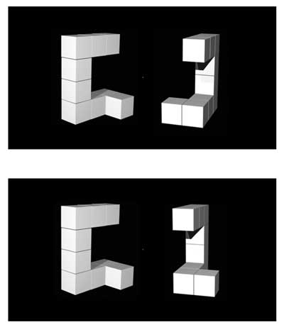
  image from Ganis and Kievit (2016)

Step 3 - plot means for each Angle condition

Note: This procedure is just one approach to create the graph in SPSS. There may be other, better ways (for this and other graphs) and you are welcome to use your preferred approach.

• The first plot we will make is a simple bar chart of mean response times, with one bar for each "Angle" level.

• To do this, first we will make a new dataset where we aggregate across trials, so that for each participant we have an average response time for each of the 4 conditions (4 rows per participant in the new datafile)

  • Use the Data->Aggregate feature to create the new dataset
  • Enter Participant & Angle as the "break" variables
  • Enter Time in the "Summaries of Variable(s)" box
  • "MEAN" is used as the aggregating function by default
  • Select "Create a new dataset containing only the aggregated variables" and enter a descriptive name like "mental-rotation-agg-bysubj"
  • check the box to sort the file before aggregating
  • When you click "OK" you will get a new datafile, you can save it with the same filename you used to name the dataset - make sure you keep this dataset as the active dataset while doing the next steps
  • go to the Variable View, and enter "response time" as the label for Time_mean

• Now, with the aggregated dataset active, go to Graphs->Chart Builder

  • First select the "simple bar" chart by dragging it from the bottom "Gallery" tab to the top Preview area (the area that says "drag a Gallery chart here")
  • Now drag the Angle variable to the x-axis of the bar chart in the preview window
  • Now drag the Time_mean variable to the y-axis of the bar chart in the preview window
  • Click OK

• Does the bar chart look how you expected? What does it tell you about the pattern of results?

Error bars

• Okay, so we can see the means, but there's no information at all about variability, so let's at least put error bars on the bar plot.
• Go back to the Chart Builder (Graphs->Chart Builder) and this time check the box for "Display error bars", and specify that you want 95% confidence intervals (now click okay)
• What do the error bars tell you in this new chart?

Show the means in a line plot

• In some cases you might prefer a point and line plot instead of bars
• Go back to the Chart Builder (Graphs->Chart Builder) and this time find the "Simple Line" plot in the Gallery and drag it to the preview window.
  • drag the Angle and Time_mean variables to the x and y axes as you did before, and select the same error bars
• Does this plot show you anything different than the bar plot?

Step 4 - group the bar plot by "DesiredResponse"

• The column "DesiredResponse" (in the unaggregated file) indicates whether the target shape was the same or different than the reference shape. Let's treat the data like a 2x4 design and split each bar into two (one bar for "same" and one for "different").

• to accomplish this, first we have to re-do the aggregation step to also group by "DesiredResponse" values

• re-activate the first (unaggregated) dataset by clicking on it or selecting it through the "window" menu of SPSS

• Now, do the same aggregation step as before (Data->Aggregate), but this time include Participant, Angle, and DesiredResponse as the "break" variables

  • Select "Create a new dataset containing only the aggregated variables" and enter a descriptive name like "mental-rotation-agg-bysubj-and-desresp"
  • When you click "OK" you will get a new datafile, you can save it with the same filename you used to name the dataset - make sure you keep this dataset as the active dataset while doing the next steps
  • go to the Variable View, and enter "response time" as the label for Time_mean

• Now, with the newly aggregated dataset active, go to Graphs->Chart Builder

  • First select the "Clustered bar" chart type by dragging it from the bottom "Gallery" tab to the top Preview area
  • Now drag the Angle variable to the x-axis of the bar chart in the preview window
  • Now drag the Time_mean variable to the y-axis of the bar chart in the preview window
  • Now drag the DesiredResponse variable to the "Cluster on X: set color" box in the preview window
  • set the error bars for 95% confidence intervals
  • Click OK

• What does this new chart tell you about the data?

Now see if you can chart the same information using a line plot instead of a bar plot

• make sure the newly aggregated dataset is the active one
• go back to the chart builder and change the chart type
  • use the "Multiple Lines" chart type and specify the x, y, and cluster variables as before

---

Step 5 - visualize a relationship between 2 variables

• Is reaction time related to accuracy?
• Let's compute accuracy for each subject, by counting the proportion of "Correct" values in the "CorrectResponse" column. We exclude trials with no response. Alternatively, you might have reasons to include these trials as incorrect for the accuracy calculation, but for this activity we will exclude them.
• Go back to the original unaggregated dataset (where each row is a single trial)
• First, select only cases that have a valid response time (Data->Select Cases, "If condition is satisfied", specify "Time > 0" for the condition
• Now aggregate the data, similarly to how you did the first time, but in addition to "Time" in the "Summaries of Variables" box, add "CorrectResponse"
  • because "CorrectResponse" is a nominal variable, you can't use MEAN as the aggregating function - instead you will use the PIN function (stands for "Percent IN")
  • to specify the aggregating function, first highlight the "CorrectResponse..." entry in the "Summaries of Variables" box, then click the "Function" button
  • now select "Percentages", "Inside", and type "Correct" (without the quotes, but match the upper/lowercase letters exactly) into both the "Low" and "High" text boxes
  • Select "Create a new dataset containing only the aggregated variables" and enter a descriptive name like "mental-rotation-agg-bysubjwithaccuracy"
  • check the box to sort the file before aggregating
  • When you click "OK" you will get a new datafile, you can save it with the same filename you used to name the dataset - make sure you keep this dataset as the active dataset while doing the next steps
• Look at the newly aggregated dataset (use the "Window" menu if you don't see it on your screen) - there should be 1 row per subject, and 3 columns (Participant, Time_mean, and CorrectResponse_pin)
• go to the Variable View, and enter "response time" as the label for Time_mean, and "accuracy" as the label for CorrectResponse_pin

Now make a scatter plot of accuracy against response time

• make sure the newly aggregated dataset is the active one

• Graphs->Chart Builder

  • drag the Scatter Plot chart type into the preview window
  • put accuracy on the x-axis and response time on the y-axis
  • include a linear trend line by checking the "total" box under "Linear Fit Lines"

• Take a look at the scatter plot - is there any relation between the two variables?

Scatter plot of response time by accuracy, grouped by DesiredResponse

• What if we wanted to split up subject RT and accuracy by DesiredResponse (whether the shapes were same or different)?
• We need to re-aggregate the data by going back to the un-aggregated dataset, and this time specifying DesiredResponse as an additional "break" variable (everything else as you had it last time)
• try it now (make sure you have excluded "no response" trials) - you should now get a new dataset with 2 rows for each subject
• set labels for the variables in the newly aggregated dataset
• Graphs->Chart Builder, use the same Scatter Plot chart type
• put accuracy on the x-axis and response time on the y-axis
• drag DesiredResponse to the "set Color" box in the preview window
• click on "Subgroups" below "Linear Fit Lines" to get trendlines for the two conditions
• Does this new chart show you anything new about the relation between accuracy and response time?

---

That's all for the SPSS activity - save your notes and move on to the R/RStudio activity when you are ready